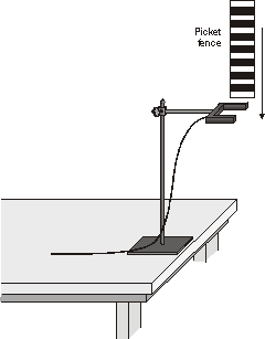
Picket Fence Free Fall
We say an object is in free fall when the only force acting on it is the earth’s gravitational force. No other forces can be acting; in particular, air resistance must be either absent or so small as to be ignored. When the object in free fall is near the surface of the earth, the gravitational force on it is nearly constant. As a result, an object in free fall accelerates downward at a constant rate. This acceleration is usually represented with the symbol g.
Physics students measure the acceleration due to gravity using a wide variety of timing methods. In this experiment, you will have the advantage of using a very precise timer connected to the calculator and a Photogate. The Photogate has a beam of infrared light that travels from one side to the other. It can detect whenever this beam is blocked. You will drop a piece of clear plastic with evenly spaced black bars on it, called a Picket Fence. As the Picket Fence passes through the Photogate, the LabPro or CBL 2 interface will measure the time from the leading edge of one bar blocking the beam until the leading edge of the next bar blocks the beam. This timing continues as all eight bars pass through the Photogate. From these measured times, the program will calculate the velocities and accelerations for this motion and graphs will be plotted.

Figure 1
objective
· Measure the acceleration of a freely falling body (g) to better than 0.5% precision using a Picket Fence and a Photogate.
Materials
|
LabPro or CBL 2 interface |
Vernier Photogate |
|
TI Graphing Calculator |
Picket Fence |
|
rogram |
clamp or ring stand to secure Photogate |
Preliminary questions
1. Inspect your Picket Fence. You will be dropping it through a Photogate to measure g. The distance, measured from one edge of a black band to the same edge of the next band, is 5.0 cm. What additional information will you need to determine the average speed of the Picket Fence as it moves through the Photogate?
2. If an object is moving with constant acceleration, what is the shape of its velocity vs. time graph?
3. Does the initial velocity of an object have anything to do with its acceleration? For example, compared to dropping an object, if you throw it downward would the acceleration be different after you released it?
Procedure
1. Fasten the Photogate rigidly to a ring stand so the arms extend horizontally, as shown in Figure 1. The entire length of the Picket Fence must be able to fall freely through the Photogate. To avoid damaging the Picket Fence, make sure it has a soft landing surface.
2. Connect the Photogate to the DIG/SONIC 1 input of the LabPro or the input on the CBL 2. Use the black link cable to connect the interface to the TI Graphing Calculator. Firmly press in the cable ends.
3. Turn on the calculator and start the DATAGATE program.
4. Set up the calculator for motion timing.
a. Select from the main screen.
b. Select from the screen.
c. Select from the screen.
d. Select from the screen.
5. Now collect your free fall data. To do this, select . Wait for the interface to beep.
6. Hold the top of the Picket Fence and drop it through the Photogate, releasing it from your grasp completely before it enters the Photogate. Be careful when releasing the Picket Fence. It must not touch the sides of the Photogate as it falls and it needs to remain vertical.
7. Press ![]() to examine your distance vs. time graph. Sketch the
graph on paper for later use. Press
to examine your distance vs. time graph. Sketch the
graph on paper for later use. Press ![]() to return to the menu.
to return to the menu.
8. Press
![]() to select and press
to select and press
![]() . Examine your velocity vs. time graph. The slope of a
velocity vs. time graph is a measure of acceleration. If the velocity
graph is approximately a straight line of constant slope, the acceleration is
constant. If the acceleration of your Picket Fence appears constant, fit a
straight line to your data.
. Examine your velocity vs. time graph. The slope of a
velocity vs. time graph is a measure of acceleration. If the velocity
graph is approximately a straight line of constant slope, the acceleration is
constant. If the acceleration of your Picket Fence appears constant, fit a
straight line to your data.
a.
Press ![]() , and select from the
screen.
, and select from the
screen.
b. Select from the main screen.
c. Select from the screen.
d. Select from the screen.
e. Record the slope of the fitted line in the Data Table.
f.
Press ![]() to see the fitted line with your data.
to see the fitted line with your data.
g.
To return to the main screen, press ![]() , and then select , finally
selecting .
, and then select , finally
selecting .
9. To establish the reliability of your slope measurement, repeat Steps 6 through 9 five more times. Do not use drops in which the Picket Fence hits or misses the Photogate. Record the slope values in the Data Table.
Data Table
|
Trial |
1 |
2 |
3 |
4 |
5 |
6 |
|
Slope (m/s2) |
|
|
|
|
|
|
|
|
Minimum |
Maximum |
Average |
|
|
Acceleration (m/s2) |
|
|
|
|
|
|
|
|||
|
Acceleration due to gravity, g |
± m/s2 |
|||
|
Precision |
% |
|||
Analysis
1. From your six trials, determine the minimum, maximum, and average values for the acceleration of the Picket Fence. Record them in the Data Table.
2. Describe in words the shape of the distance vs. time graph for the free fall of the picket fence.
3. Describe in words the shape of the velocity vs. time graph. How is this related to the shape of the distance vs. time graph?
4. The average acceleration you determined represents
a single best value, derived from all your measurements. The minimum and maximum
values give an indication of how much the measurements can vary from trial to
trial; that is, they indicate the precision of your measurement. One way of
stating the precision is to take half of the difference between the minimum and
maximum values and use the result as the uncertainty of the measurement. Express
your final experimental result as the average value,
± the uncertainty. Round the
uncertainty to just one digit and round the average value to the same decimal
place.
For example, if your minimum, average, and maximum values are 9.12, 9.93, and
10.84 m/s2, express your result as g = 9.9 ± 0.9 m/s2.
Record your values in the Data Table.
5. Express the uncertainty as a percentage of the acceleration. This is the precision of your experiment. Enter the value in your Data Table. Using the example numbers from the last step, the precision would be
![]()
6. Compare your measurement to the generally accepted value of g (from a textbook or other source). Does the accepted value fall within the range of your values? If so, your experiment agrees with the accepted value.
7.
Inspect your velocity graph. How would the associated acceleration vs.
time graph look? Sketch your prediction on paper. From the main screen, select
Use the cursor keys ![]() and
and ![]() to select and press
to select and press
![]() . Comment on any differences between the calculator’s graph
and your prediction. Trace across the acceleration values using your cursor
keys. Note that the vertical scale of the graph does not include zero. Is the
variation as large as it appears?
. Comment on any differences between the calculator’s graph
and your prediction. Trace across the acceleration values using your cursor
keys. Note that the vertical scale of the graph does not include zero. Is the
variation as large as it appears?
8. Find the average acceleration from the trace values. How does this compare with the acceleration value for the same drop, determined from the slope of the velocity graph?
Extensions
1. Use the distance vs. time data and a quadratic fit to determine g.
2. Display the acceleration vs. time plot and
note the apparent variation in acceleration. Trace across the plot with the
![]() and
and ![]() cursor keys, and read the acceleration values individually.
Is the acceleration varying as much as it first appears?
cursor keys, and read the acceleration values individually.
Is the acceleration varying as much as it first appears?
3. Would dropping the Picket Fence from higher above the Photogate change any of the parameters you measured? Try it.
4. Would throwing the Picket Fence downward, but letting go before it enters the Photogate, change any of your measurements? How about throwing the Picket Fence upward? Try performing these experiments.
5. How would adding air resistance change the results? Try adding a loop of clear tape to the upper end of the Picket Fence. Drop the modified Picket Fence through the Photogate and compare the results with your original free fall results.
6. Investigate how the value of g varies around the world. For example, how does altitude affect the value of g? What other factors cause this acceleration to vary at different locations? How much can g vary at a location in the mountains compared to a location at sea level?